Get the packages

To use torch, you first need to install it. Same for its high-level wrapper, luz. While torch has all the basic functionality, luz provides a declarative, concise API that lets you train a network in a few lines of code.

To get the respective CRAN versions, do

install.packages("torch")
install.packages("luz")

Does it work? Here’s a quick test:

library(torch)
library(luz)
torch_tensor(1)

torch_tensor
 1
[ CPUFloatType{1} ]

Now, while torch contains all the core functionality, and luz, the training logic, there is a whole ecosystem built around them.

Notably, torchvision is essential to image-processing tasks. In this example, we don’t use it much – overtly, that is. It’s used more prominently behind the scenes. Let’s get it:

install.packages("torchvision")

library(torchvision)

Finally, there is an evolving package, named torchdatasets , that wraps datasets in a convenient format, rendering them immediately usable from torch. Let’s get this as well, as we’re going to use one of the datasets it provides.

remotes::install_github("mlverse/torchdatasets")

library(torchdatasets)

Get the dataset

“Guess the correlation” is a fun dataset that tasks one – a person, if they feel like, or a program, if we train it – to estimate the (linear) correlation between two variables displayed in a scatterplot.

torchdatasets will download, unpack, and preprocess it for us.

The training set is huge; it has 150000 observations. For instruction purposes, we don’t really need so much data – we’ll restrict ourselves to small subsets, for each of training, validation, and test sets.

train_indices <- 1:10000
val_indices <- 10001:15000
test_indices <- 15001:20000

Now, the following snippet does the following:

download and unpack the dataset,
do some custom preprocessing on the images (on top of what is already done by default) – more on that soon

take just the first 10000 observations and put them in a torch Dataset object named train_ds.

add_channel_dim <- function(img) img$unsqueeze(1)
crop_axes <- function(img) transform_crop(img, top = 0, left = 21, height = 131, width = 130)

root <- file.path(tempdir(), "correlation")

train_ds <- guess_the_correlation_dataset(
# where to unpack
root = root,
# additional preprocessing 
transform = function(img) crop_axes(img) %>% add_channel_dim(),
# don't take all data, but just the indices we pass in
indexes = train_indices,
download = TRUE
)

As we’re at it, let’s do the same for the validation and test sets. We don’t need to download again, as we’re building on the same underlying data. We just pick different observations.

valid_ds <- guess_the_correlation_dataset(
    root = root,
    transform = function(img) crop_axes(img) %>% add_channel_dim(),
    indexes = val_indices,
    download = FALSE
  )

test_ds <- guess_the_correlation_dataset(
    root = root,
    transform = function(img) crop_axes(img) %>% add_channel_dim(),
    indexes = test_indices,
    download = FALSE
  )

Let’s counter-check we got what we wanted. How many items are there in each set?

length(train_ds)
length(valid_ds)
length(test_ds)

[1] 10000
[1] 5000
[1] 5000

And how does a single observation look like? Here is the first one:

train_ds[1]

$x
torch_tensor
(1,.,.) = 
 Columns 1 to 9  0.9999  0.9999  0.9999  0.9999  0.9999  0.9999  0.9999  0.9999  0.9999
  0.0000  0.0000  0.0000  0.0000  0.0000  0.0000  0.0000  0.0000  0.0000
  0.0000  0.9999  0.9999  0.9999  0.9999  0.9999  0.9999  0.9999  0.9999
  0.0000  0.9999  0.9999  0.9999  0.9999  0.9999  0.9999  0.9999  0.9999
  0.0000  0.9999  0.9999  0.9999  0.9999  0.9999  0.9999  0.9999  0.9999
  0.0000  0.9999  0.9999  0.9999  0.9999  0.9999  0.9999  0.9999  0.9999
  0.0000  0.9999  0.9999  0.9999  0.9999  0.9999  0.9999  0.9999  0.9999
  0.0000  0.9999  0.9999  0.9999  0.9999  0.9999  0.9999  0.9999  0.9999
  0.0000  0.9999  0.9999  0.9999  0.9999  0.9999  0.9999  0.9999  0.9999
  0.0000  0.9999  0.9999  0.9999  0.9999  0.9999  0.9999  0.9999  0.9999
  0.0000  0.9999  0.9999  0.9999  0.9999  0.9999  0.9999  0.9999  0.9999
  0.0000  0.9999  0.9999  0.9999  0.9999  0.9999  0.9999  0.9999  0.9999
  0.0000  0.9999  0.9999  0.9999  0.9999  0.9999  0.9999  0.9999  0.9999
  0.0000  0.9999  0.9999  0.9999  0.9999  0.9999  0.9999  0.9999  0.9999
  0.0000  0.9999  0.9999  0.9999  0.9999  0.9999  0.9999  0.9999  0.9999
  0.0000  0.9999  0.9999  0.9999  0.9999  0.9999  0.9999  0.9999  0.9999
  0.0000  0.9999  0.9999  0.9999  0.9999  0.9999  0.9999  0.9999  0.9999
  0.0000  0.9999  0.9999  0.9999  0.9999  0.9999  0.9999  0.9999  0.9999
  0.0000  0.9999  0.9999  0.9999  0.9999  0.9999  0.9999  0.9999  0.9999
  0.0000  0.9999  0.9999  0.9999  0.9999  0.9999  0.9999  0.9999  0.9999
  0.0000  0.9999  0.9999  0.9999  0.9999  0.9999  0.9999  0.9999  0.9999
  0.0000  0.9999  0.9999  0.9999  0.9999  0.9999  0.9999  0.9999  0.9999
  0.0000  0.9999  0.9999  0.9999  0.9999  0.9999  0.9999  0.9999  0.9999
  0.0000  0.9999  0.9999  0.9999  0.9999  0.9999  0.9999  0.9999  0.9999
  0.0000  0.9999  0.9999  0.9999  0.9999  0.9999  0.9999  0.9999  0.9999
  0.0000  0.9999  0.9999  0.9999  0.9999  0.9999  0.9999  0.9999  0.9999
  0.0000  0.9999  0.9999  0.9999  0.9999  0.9999  0.9999  0.9999  0.9999
  0.0000  0.9999  0.9999  0.9999  0.9999  0.9999  0.9999  0.9999  0.9999
  0.0000  0.9999  0.9999  0.9999  0.9999  0.9999  0.9999  0.9999  0.9999
... [the output was truncated (use n=-1 to disable)]
[ CPUFloatType{1,130,130} ]

$y
torch_tensor
-0.45781
[ CPUFloatType{} ]

$id
[1] "arjskzyc"

It’s a list of three items, the last of which we’re not interested in for our purposes.

The second, a scalar tensor, is the correlation value, the thing we want the network to learn. The first, x, is the scatterplot: a tensor representing an image of dimensionality 130*130. But wait – what is that 1 in the shape output?

[ CPUFloatType{1,130,130} ]

This really is a three-dimensional tensor! The first dimension holds different channels – or the single channel, if the image has but one. In fact, the reason x came in this format is that we requested it, here:

add_channel_dim <- function(img) img$unsqueeze(1)

train_ds <- guess_the_correlation_dataset(
    # ...
    transform = function(img) crop_axes(img) %>% add_channel_dim(),
    # ...
  )

add_channel_dim() was passed in as a custom transformation, to be applied to every item of the dataset. It calls one of torch’s many tensor operations, unsqueeze(), that adds a singleton dimension at a requested position.

How about the second custom transformation?

crop_axes <- function(img) transform_crop(img, top = 0, left = 21, height = 131, width = 130)

Here, we crop the image, cutting off the axes and labels on the left and bottom. These image regions don’t contribute any distinctive information, and having the images be smaller saves memory.

Work with batches

Now, we’ve done so much work already, but you haven’t actually seen any of the scatterplots yet! The reason we’ve been waiting until now is that we want to show a bunch of them at a time, and for that, we need to know how to handle batches of data.

So let’s create a DataLoader object from the training set. We’ll soon use it to train the model, but right now, we’ll just plot the first batch.

A DataLoader needs to know where to get the data – namely, from the Dataset it gets passed –, as well as how many items should go in a batch. Optionally, it can return data in random order (shuffle = TRUE).

train_dl <- dataloader(train_ds, batch_size = 64, shuffle = TRUE)

Like a Dataset, we can query a DataLoader for its length. For the Dataset, this meant number of items; for a DataLoader , it means number of batches:

length(train_dl)

[1] 157

To access the first batch, we create an iterator from the DataLoader and ask it for the first batch. Even if it weren’t for plotting, you might do this just to check that the dimensions look ok:

batch <- dataloader_make_iter(train_dl) %>% dataloader_next()

dim(batch$x)
dim(batch$y)

[1]  64   1 130 130
[1] 64

And plot! Note how we first remove the channels dimension – as.raster() wouldn’t like it – and then, convert the tensor to R for further processing:

par(mfrow = c(8,8), mar = rep(0, 4))

images <- as.array(batch$x$squeeze(2))

images %>%
  purrr::array_tree(1) %>%
  purrr::map(as.raster) %>%
  purrr::iwalk(~{plot(.x)})

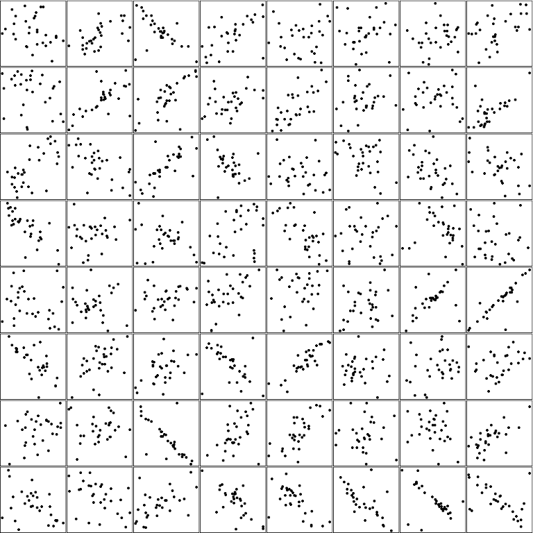
Want to try your skill at guessing these? Here is the corresponding ground truth:

batch$y %>% as.numeric() %>% round(digits = 2)

[1] -0.29  0.58 -0.57  0.56  0.10  0.09  0.21  0.45 -0.24  0.65  0.70  0.40  0.71  0.20  0.07  0.66  0.65 -0.56  0.73
[20] -0.40 -0.18 -0.42 -0.46 -0.45 -0.77  0.09 -0.19  0.40 -0.70 -0.04 -0.16 -0.13 -0.18  0.01  0.25  0.54  0.21  0.28
[39]  0.49  0.86 -0.70  0.51  0.47 -0.46  0.88  0.00  0.24  0.28  0.28 -0.04 -0.74  0.43  0.74  0.01 -0.21  0.66 -0.45
[58] -0.44  0.50 -0.69 -0.65 -0.66 -0.55 -0.53

Now, just as they got their own Dataset objects, test and validation data each need their own DataLoader.

valid_dl <- dataloader(valid_ds, batch_size = 64)
length(valid_dl)

[1] 79

test_dl <- dataloader(test_ds, batch_size = 64)
length(test_dl)

[1] 79

And we’re ready to create the model!

Create the model

Let’s first see what we’re trying to accomplish. Our input data are images; normally this means we’ll work with some kind of convolutional neural network (CNN). In torch, a neural network is a module: a container for more granular modules, which themselves may be built up of yet more fine-grained modules. While in theory, this kind of compositionality is unlimited, in our example there are just two levels: a top-level module representing the model, and submodules that, in other frameworks, would be called layers.

The overall model is created by a call to nn_module(). This instantiates an nn_Module, an R6 class that knows how to act as a neural network. This object can have any number of methods, but two are essential:

initialize(), the place to instantiate any submodules; and
forward(), the place to define what should happen when this module is called.

In initialize() , we instantiate five submodules – two convolutional layers and two linear ones:

# zooming in on just initialize() - don't run standalone

net <- nn_module(
  
  # ...
  
  initialize = function() {
    
    self$conv1 <- nn_conv2d(in_channels = 1, out_channels = 32, kernel_size = 3)
    self$conv2 <- nn_conv2d(in_channels = 32, out_channels = 64, kernel_size = 3)
    self$conv3 <- nn_conv2d(in_channels = 64, out_channels = 128, kernel_size = 3)
    
    self$fc1 <- nn_linear(in_features = 14 * 14 * 128, out_features = 128)
    self$fc2 <- nn_linear(in_features = 128, out_features = 1)
    
  },
  
 # ...
)

The convolutional (often abbreviated conv) layers apply a filter (or: kernel) of size 3 x 3. This filter slides over the image and computes local aggregates. In fact, there is not just a single filter, there are:

32 of them in the first conv layer,
64 in the second, and
128 in the third.

The filters are trained to pick up informative spatial features, features that will be able to tell us something about the image.

In addition to the three conv layers, we have two linear ones. These are the prototypical neural network layers that get input from all units in the previous layer, combine individual contributions as they see fit, and send on their own individual results to all units in the next layer. The first linear layer will act on the features received from the last conv layer; it consists of 128 units. The second one is the output layer. It outputs a single numeric value, a value that represents the guess our network is making about the size of the correlation.

Now, while initialize() defines the layers, forward() specifies the order in which to call them – and what to do “in between”:

# zooming in on just forward() - don't run standalone

net <- nn_module(
  
 # ...
  
  forward = function(x) {
    
    x %>% 
      self$conv1() %>%
      nnf_relu() %>%
      nnf_avg_pool2d(2) %>%
      
      self$conv2() %>%
      nnf_relu() %>%
      nnf_avg_pool2d(2) %>%
      
      self$conv3() %>%
      nnf_relu() %>%
      nnf_avg_pool2d(2) %>%
      
      torch_flatten(start_dim = 2) %>%
      self$fc1() %>%
      nnf_relu() %>%
      
      self$fc2()
  }
)

What are these things that happen “in between”? In fact, they are of different types.

Firstly, we have nnf_relu(), called three times: after each of the conv layers and after the first linear layer. This is a so-called activation function – a function that takes the raw results computed by a layer and performs some operation on them. In the case of nnf_relu() (ReLU - Rectified Linear Unit) what it does is leave positive values alone while setting negative ones to 0. You’ll encounter additional activation functions when you continue your torch journey, but ReLU is among the very-most-in-use ones today.

Secondly, we have nnf_avg_pool2d(2) , called after each conv layer. This function downsizes the image, replacing a 2 x 2 patch of pixels by its average. So while we’re going up in the number of channels (from 1 via 32 and 64 to 128), we decrease spatial resolution.

Thirdly, there is torch_flatten(). This one doesn’t compute anything - it just reshapes its inputs, going – in this case – from a four-dimensional structure outputted by the second conv layer to the two-dimensional one expected by the first linear layer.

Now, here is the complete model creation code:

torch_manual_seed(777)

net <- nn_module(
  
  "corr-cnn",
  
  initialize = function() {
    
    self$conv1 <- nn_conv2d(in_channels = 1, out_channels = 32, kernel_size = 3)
    self$conv2 <- nn_conv2d(in_channels = 32, out_channels = 64, kernel_size = 3)
    self$conv3 <- nn_conv2d(in_channels = 64, out_channels = 128, kernel_size = 3)
    
    self$fc1 <- nn_linear(in_features = 14 * 14 * 128, out_features = 128)
    self$fc2 <- nn_linear(in_features = 128, out_features = 1)
    
  },
  
  forward = function(x) {
    
    x %>% 
      self$conv1() %>%
      nnf_relu() %>%
      nnf_avg_pool2d(2) %>%
      
      self$conv2() %>%
      nnf_relu() %>%
      nnf_avg_pool2d(2) %>%
      
      self$conv3() %>%
      nnf_relu() %>%
      nnf_avg_pool2d(2) %>%
      
      torch_flatten(start_dim = 2) %>%
      self$fc1() %>%
      nnf_relu() %>%
      
      self$fc2()
  }
)

Even before training, we can call the model on a batch of data – this immediately tells us if we got all shapes matching up:

model <- net()
model(batch$x)

torch_tensor
0.01 *
-2.8979
 -2.8873
 -2.8699
 -2.9787
 -2.8223
 -3.0255
 -3.1181
 -3.0603
 -3.0520
 -2.8242
 -3.0000
 -2.9150
 -2.9497
 -2.7662
 -2.7980
 -2.9540
 -2.8548
 -2.7927
 -3.0426
 -2.9540
 -2.8846
 -2.8008
 -2.8966
 -2.8358
 -2.9266
 -2.9022
 -2.8667
 -2.8716
 -2.7371
... [the output was truncated (use n=-1 to disable)]
[ CPUFloatType{64,1} ]

After all that hard work, training the model with luz is a breeze.

Train the network

What happens when you train a neural network? Conceptually, the following has to happen for every batch. (Wait – don’t execute these lines :-) You’ll see luz taking care of it for you in a minute.)

Run the model on the input, to obtain its current predictions:
```
output <- model(b$x)
```
Calculate the loss, a measure of divergence between model estimate and ground truth:
```
loss <- nnf_mse_loss(output, b$y$unsqueeze(2))
```
Have that loss propagate back through the network, causing gradients to be computed for all parameters:
```
loss$backward()
```
Ask the optimizer to update the parameters accordingly:
```
optimizer$step()
```

Fortunately, with luz, we don’t have to compute the training loop ourselves! All this is taken care of by a pair of two functions: setup() and fit().

In setup(), we decide which loss function and which optimization algorithm to use. For regression problems, the most popular loss is mean squared error: nn_mse_loss().

And among optimization algorithms (“optimizers”), among the most popular ones is Adam (optim_adam()).

setup() is called on the model definition, like so:

fitted <- net %>%
  setup(
    loss = function(y_hat, y_true) nnf_mse_loss(y_hat, y_true$unsqueeze(2)),
    optimizer = optim_adam
  )

Then fit() is used to pass the training data loader, the number of epochs to train for, and optionally, the validation data loader. After every epoch, the model is run on the validation data, in “test mode” (no parameter updates involved). That way, you immediately see whether you’re overfitting to the training set. Here are both calls together – everything we need to start training:

fitted <- net %>%
  setup(
    loss = function(y_hat, y_true) nnf_mse_loss(y_hat, y_true$unsqueeze(2)),
    optimizer = optim_adam
  ) %>%
  fit(train_dl, epochs = 10, valid_data = test_dl)

As you can see, the network has made good progress – on both training and validation set. How about the test set? And how good of a fit are the inferred correlations?

Evaluate performance

We use luz::predict() to get predictions on the test set:

preds <- predict(fitted, test_dl)

How do predictions and ground truth line up? Well, since all this has been about scatterplots, why not create one to investigate that?

preds <- preds$to(device = "cpu")$squeeze() %>% as.numeric()
test_dl <- dataloader(test_ds, batch_size = 5000)
targets <- (test_dl %>% dataloader_make_iter() %>% dataloader_next())$y %>% as.numeric()

df <- data.frame(preds = preds, targets = targets)

library(ggplot2)

ggplot(df, aes(x = targets, y = preds)) +
  geom_point(size = 0.1) +
  theme_classic() +
  xlab("true correlations") +
  ylab("model predictions")

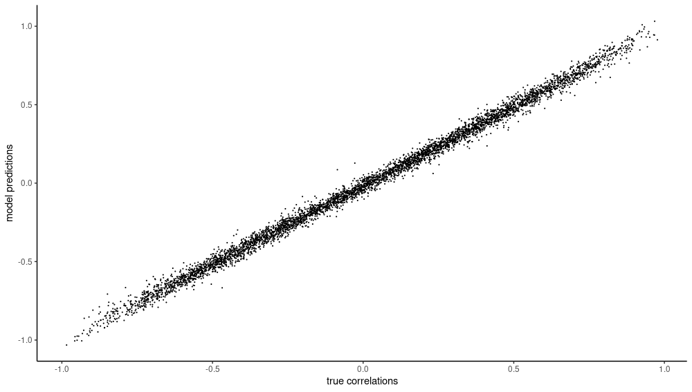
Want to guess the correlation …?

So that’s it - you’ve seen the complete workflow end-to-end, from data loading to model evaluation. The next tutorial asks a few what if? questions – e.g., what if I don’t want to predict a numerical output? – and offers some ideas for experimentation.